The Comfort Zone Loop

Finding ones comfort zone is like a winding road, with ever-changing challenges and rewards. This first blog post gives a glimpse into my experience of finding my comfort zone in programming as part of my academic and professional careers, and how my definition of this comfort zone has changed over the years.

When I first started writing code in a first-year computer science course on Java, I will admit... I failed miserably. It required such a different way of thinking that I just was not used to. I felt like I was going to have to pull out all the stops to pass this course, let alone write efficient, elegant code. Even tasks considered trivial, such as printing a pattern of characters onto the screen, I could not accomplish. My mind simply could not envision the series of operations that were required to achieve these tasks. In fact, it took me the better part of a year to learn how to use and construct loops.

Fast forward 7 years, I am part of an incredibly talented team at an industry-leading company and responsible for most of the software development in our department. Using loops has become my comfort zone and feels like a second nature. Not only is it easy to envision the solution to a problem in the form of (often nested) loops, but it also makes the resulting code extremely easy to read and understand; something that becomes increasingly important when developed code needs to be justified or modified months later.

This is all great when the operations performed inside the loop are relatively quick and the number of iterations is manageable. However, this quickly caught up with me when the software tools I was developing became more advanced, with more features, and had to compute large data sets which required tens of thousands of loop iterations. The execution time of my code went from a comfortable few minutes, to perhaps a few hours, to days and, eventually, weeks.

To give a simple example, let us imagine a scenario where you want to compute the sum of the elements of every row in a matrix, M, in specific columns only, as shown below:

Generating a matrix S as the sum of columns 2, 3, 5, 7, 8, 9 in each row of matrix M

One way of achieving this would be to write a for-loop which iterates from 1 to the number of rows in the input matrix, M. At each iteration, the sum of the elements in the desired columns is computed, and stored in the corresponding row of an output matrix, S. In Matlab, if the matrix, M, has 100 rows, this would look something like:

% Generate the input matrix, M
M = rand(100,10);
% Generate the matrix, C, with the desired column indices
C = [2 3 5 7 8 9];
% Compute the sum across the desired columns for each row in M
tic
for i = 1:size(M,1)
    S(i,1) = sum(M(i,C));
end
toc

The resulting matrix, S, is a 100 x 1 matrix and the total execution time is around 1 millisecond. However, let us now fast-forward to a scenario where you are dealing with much larger data sets and M becomes a matrix with 10 million rows. Executing the same for-loop, you'll see an increase in execution time of 10,000 times or more!

% Generate the input matrix, M
M = rand(10000000,10);
% Generate the matrix, C, with the desired column indices
C = [2 3 5 7 8 9];
% Compute the sum across the desired columns for each row in M
tic
for i = 1:size(M,1)
    S_slow(i,1) = sum(M(i,C));
end
toc

As you can imagine, the operations to perform inside the loop can get much more complex than this and, needless to say, I had to re-think the way I was writing code as a whole. Once again, I had to change my way of thinking and teach my brain to envision the solution to a problem in a completely different way. Once again, I had to step out of my comfort zone and explore a new unknown. This did not mean a complete ban on loops, far from actually, but I had to be smart about when I would use loops and develop an alternative solution when the number of required iterations would become too large. It turns out that this alternative solution comes in the form of vectorizing the problem space and leveraging the power of matrix operations.

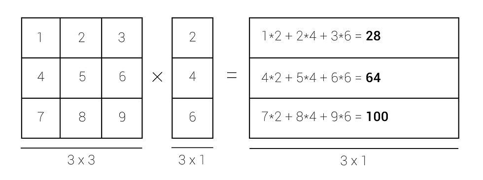
To illustrate the advantage of matrix operations in our simple example, let us take that same 10,000,000 x 10 matrix, M. Rather than using a for-loop to compute the desired sum for each row of the matrix, we could instead use the properties of matrix multiplication to our advantage. Recall that the rules of matrix multiplication are as follows:

Illustrating the rules of matrix multiplication

Therefore, we can construct a binary 10 x 1 matrix, C, which represents the indices of the columns for which we would like to compute the sum (i.e. columns 2, 3, 5, 7, 8 and 9) and multiply this with our matrix, M. In Matlab, this would look something like:

% Generate a binary matrix, C, with a 1 at indices 2, 3, 5, 7, 8, 9
C = [0;1;1;0;1;0;1;1;1;0];
% Compute the sum across the desired columns for each row in M
tic
S_fast = M * C;
toc
isequal(S_slow, S_fast)

While the resulting matrix, S_fast, is identical to the previously-computed matrix, S_slow, the execution time will be about 250 times faster! Replacing the for-loop with matrix multiplication, in this example, will reduce the execution time from about 10 seconds to just a few milliseconds. This realization that re-thinking my problem space could have such a dramatic impact on the efficiency and execution time of my code, opened up a whole new set of possibilities for me. On this blog, I would like to share with you the various ideas and concepts I have discovered since then and the ones I continue to discover along the way.